qrm-logger

A software-defined radio (SDR) application for monitoring and logging radio frequency interference in amateur radio bands, based on GNU Radio.

Both QRM, “Are you being interfered with?” and QRN, “Are the atmospherics strong?” are still common abbreviations used in Amateur Radio. Today, QRM stands for human-made noise, as opposed to QRN, which indicates noise from natural sources. If you hear an operator say, “I’m getting some QRM,” it means there’s man-made interference affecting your transmission. **

     

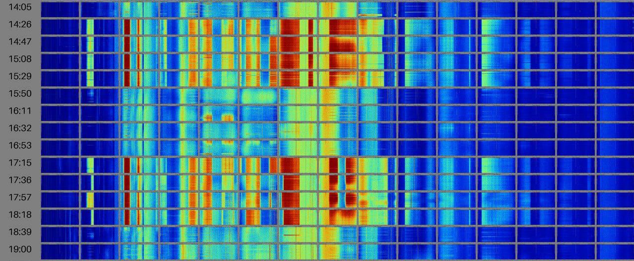
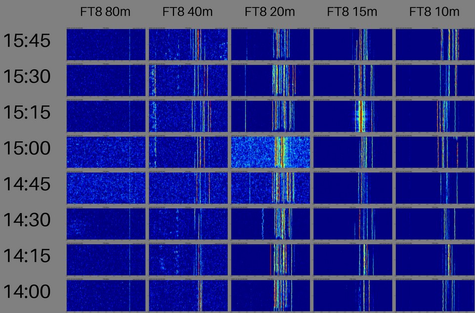
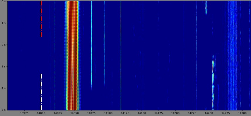
The image above shows an example for strong periodic QRM at my QTH. Each image in the grid is a 2 MHz wide recording, covering 0 - 30 MHz in total. These recordings were captured using an RTL‑SDR v4 (It is quite likely that the plots show phantom signals in addition to the main QRM due to overloading)

Purpose of this application

Periodic broadband QRM that appears at random times is particularly challenging to identify and locate, especially on the shortwave bands. Sometimes it helps to determine the timing of the QRM to infer its source.

This tool lets you record the spectrum (either manually or at periodic intervals) and create image grids for easy analysis. It also generates RMS CSV files for further analysis.

• Optimized for Raspberry Pi (Linux); also works on Windows and macOS
• SDR support out of the box: RTL‑SDR v4 and SDRplay RSP1A (requires a 3rd‑party driver compilation step)
• Python 3.10+; requires conda/mamba with the conda‑forge channel.

Architecture:

• Backend: Python application using GNU Radio for SDR processing
• Frontend: Alpine.js single-page application served by the Python backend
• Dependencies: All frontend dependencies are included via CDN - no npm/node required
• Installation: Simply install the conda environment and run python main.py

Overview

Key Features

• Web interface: Start/stop recording; view plots, grids, and RMS.
• Multiple SDR support: Preconfigured for RTL‑SDR v4 and SDRplay RSP1A (with limitations); extensible to other GNU Radio devices.
• Visual spectrum analysis: Waterfall plots generated with Matplotlib. Single plots are combined into a daily grid view.
• Scheduler: Application-level cron scheduler for periodic recording.
• Amateur‑radio band markers: Built-in band markers for HF bands.
• CSV data export: RMS data for further analysis.

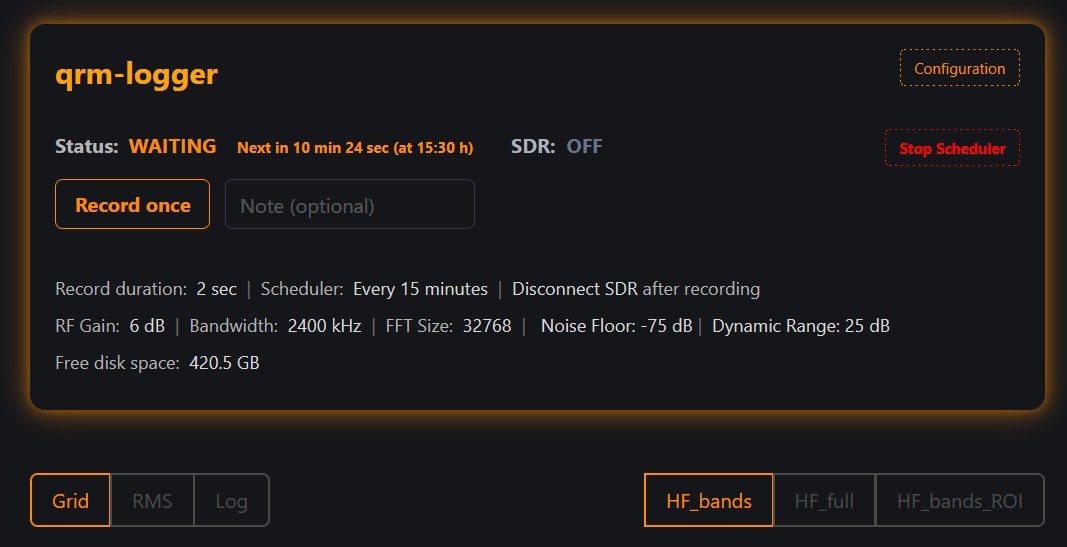
Above is a screenshot of the web UI. You can also run the application without the UI. All data is saved in a well-defined directory structure.

     

Processing Steps

Spectrum Data Capture

The application records the radio spectrum in configurable frequency slices (typically 2 MHz segments). Each slice (capture) is recorded for 2 seconds by default. There are two predefined frequency capture sets:

• HF_bands : Most common amateur radio HF bands (plots are zoomed to band boundaries, with some margin)
• HF_full : Full HF spectrum up to 30 MHz in 2 MHz steps (15 slices total)

Additional capture sets can be added in config/capture_definitions.py. A wideband set for 5 MHz captures is also available.

     

Plot each recording

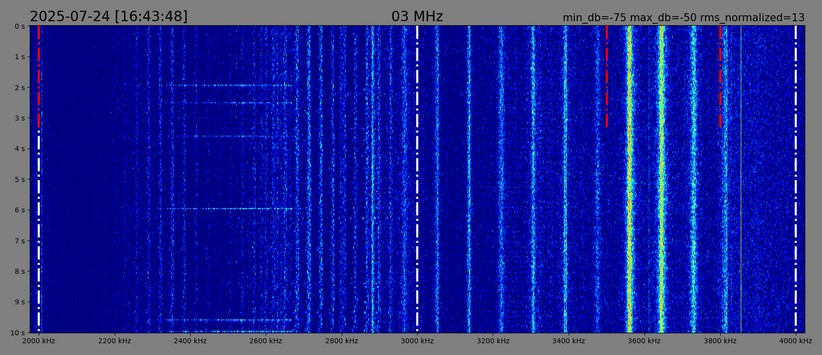
Waterfall plots are generated with Matplotlib. Harmonic interference is easy to spot. White lines are 1 MHz markers. Red lines are amateur radio band boundaries (Region 1, you can customize this in the configuration).

You can use the Browse Plots button to cycle through the individual plots in a slideshow. Use the keyboard to cycle quickly.

     

Grid Visualization

Once individual spectrum plots are generated, the application combines them into organized grid layouts. By default, two grid images per day are generated. This grid view allows for easy comparison across different frequency ranges and time periods, making it simple to identify patterns.

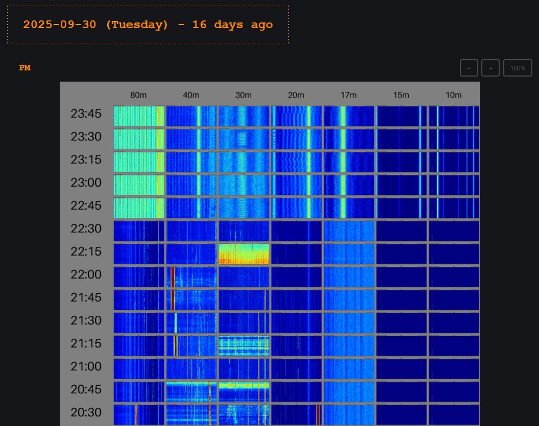
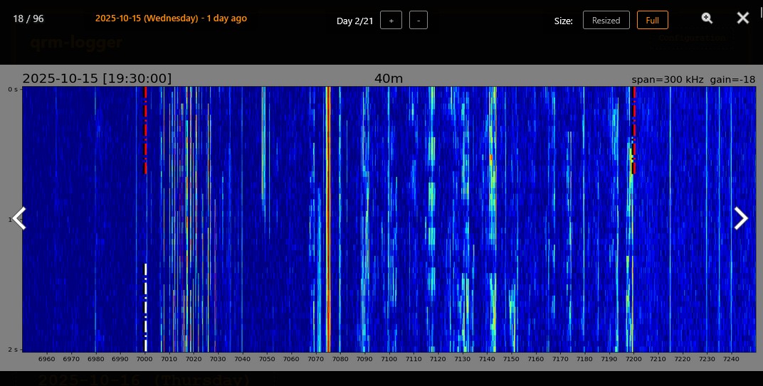
Click on the image to open the grid image zoom viewer.

The application also generates averaged plots and grids in addition to the waterfall plots and grids:

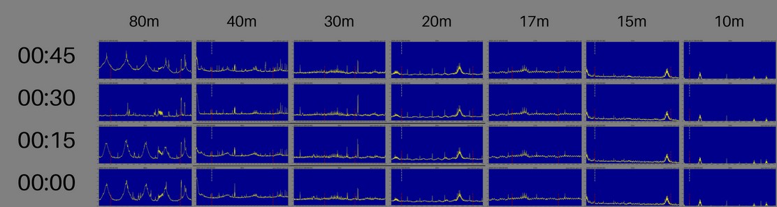
These plots show dB ranges on the scale, which makes them useful during initial calibration.

     

RMS

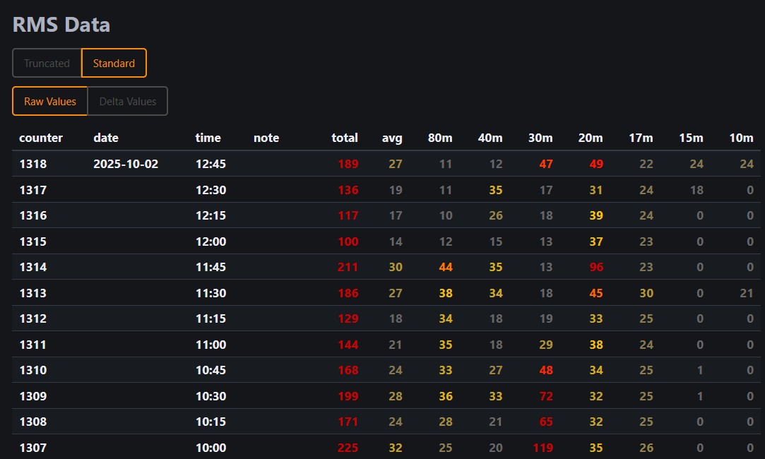
The RMS feature calculates Root Mean Square values across frequency ranges to quantify interference levels.

It provides two measurements: standard RMS (includes all signals) and truncated RMS (limits the strongest 5% of samples to reduce the impact of narrowband spikes). RMS is normalized to a percentage by linearly scaling its dB value between min_db (0%) and max_db (100%); it can exceed 100% when the signal is stronger than max_db.

Results are exported to CSV and shown with color-coded thresholds in the web UI.

     

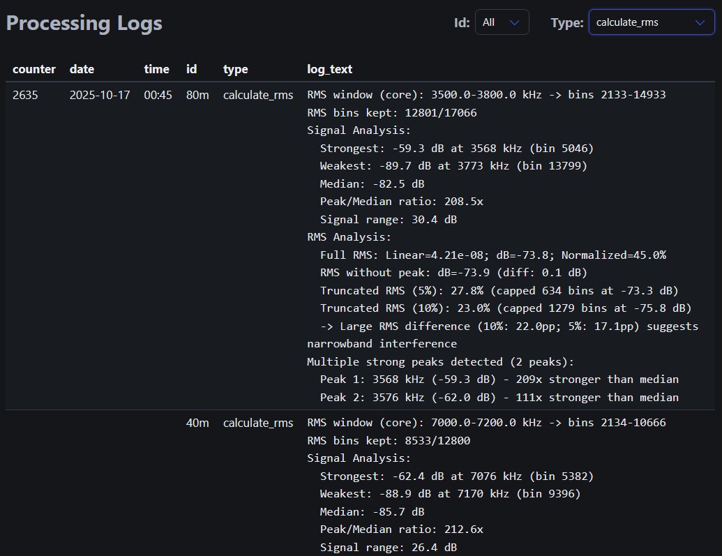
Logs

The application writes logs during processing. These can be browsed in the UI. Note that the UI displays only the logs of the two most recent days by default.

     

Regions of Interest

The ROI (Region of Interest) feature lets you define specific frequency ranges to analyze within your captured RF data. It crops FFT bins to focus on narrow bands (e.g., FT8 windows) and generates separate plots for each ROI without recapturing data. ROIs are configured in the config panel and stored as a JSON file.

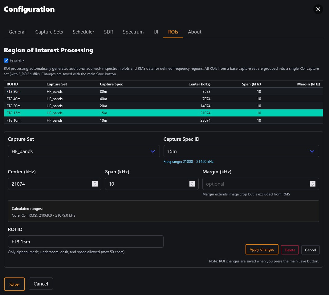
There is a preconfigured set of FT8 frequency regions. Make sure your clock is accurate, and start recording via the scheduler in order to align the timing with a FT8 cycle.

This feature is useful for getting an initial idea of the signal-to-noise ratio (SNR).

Best practices

First steps

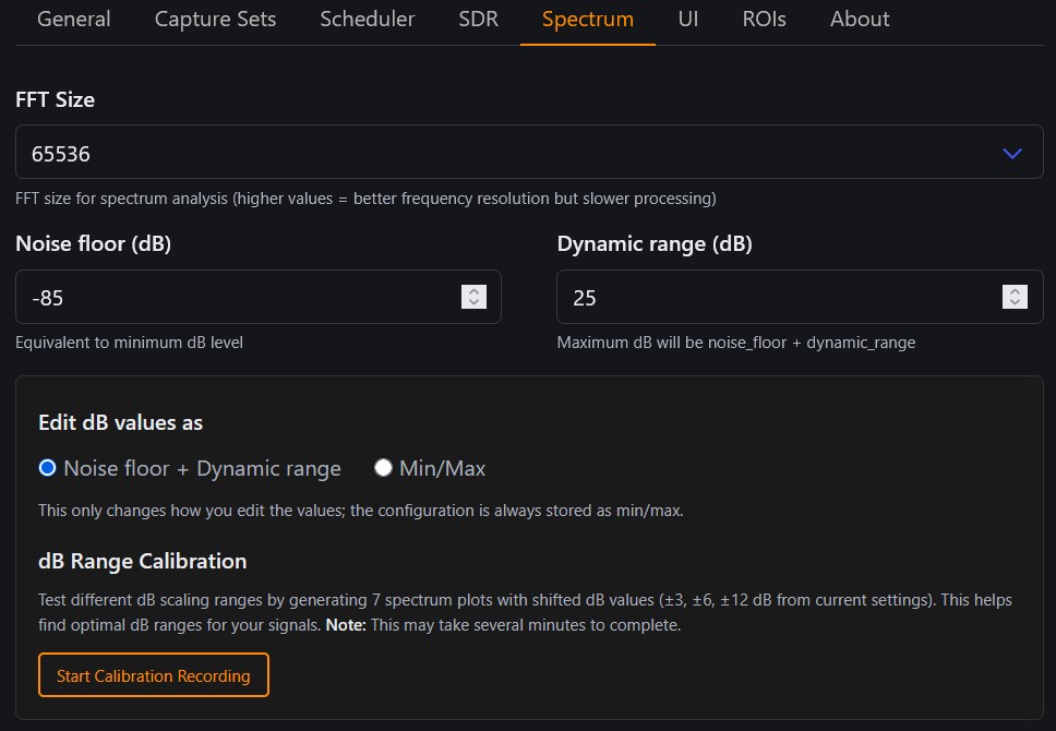
Auto Gain Control (AGC) is disabled during recording, so you must "calibrate" first by choosing a dB range for the plots and RMS calculation in the configuration screen on the spectrum tab.

Press the "Record once" button to make a recording with the default settings. Then open Grid view, switch to Average mode, and browse the plots. Check the scale on the left: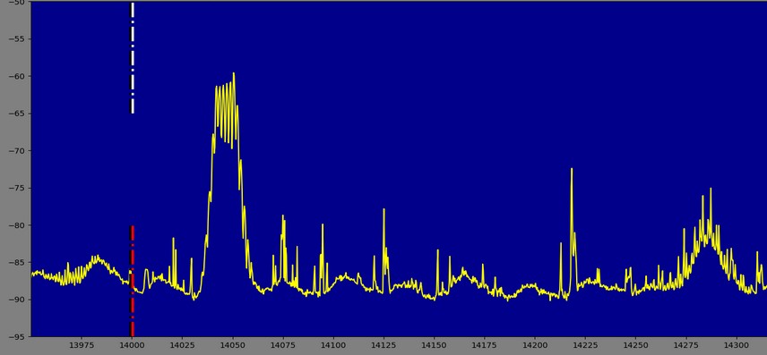

The noise floor is just below 85 dB, so this would be a good value to use for the noise‑floor dB setting. The dynamic range setting of 25 dB works quite well in most scenarios.

These settings would result in a waterfall plot like this:

You can also try the dB‑range calibration feature to generate plots with different dB settings and choose an appropriate value.

If you cannot see the noise floor in the plots, try adjusting the RF gain level in the SDR tab. Also try lowering min_db since the averaging plot minimum scale is limited to min_db - 10

Important

• Make sure your recording setup is not causing additional QRM. Try to identify which QRM (if any) is caused by your recording setup.
• In my setup, the official Raspberry Pi 4 power supply created minor broadband noise on 20 meters. I replaced it with an old Alexa power supply, which seems to be much cleaner.
• First do some recordings on battery power and/or in a location without any QRM to get baseline plots.

Operation

• A record duration of 2 seconds is sufficient to capture the noise floor and potential QRM. Note that the waterfall plot will be quite pixelated with this little amount of data. Increase to 5 or 10 seconds to detect potential pulse signals.
• Use a reasonable scheduler frequency when running the application 24/7. The default schedule (every 15 minutes) will generate images totaling at least 100 MB per day.
• You can add a note when starting a manual recording. This text will be included in the grid’s time column and in the RMS data.
• The application stores all recordings in the _recordings directory together with a counter text file. Simply rename the directory if you want to start from scratch - the application creates a new directory automatically.

RTL-SDR v4

• A bandwidth setting of 2400 kHz is recommended when using the HF_full capture set; the plots are cropped to 2 MHz to avoid filter-edge roll-off and sidelobes at the band edges.
• For the HF_bands set, choose a custom bandwidth of 1024 kHz in the "Capture Sets" config tab.

SDRPlay RSP1A

• You will have to compile the driver first. Then uncomment the HF_full_wide capture set in config/capture_definitions.py and enable it in the UI.
• This capture set crops to 5 MHz span slices and works well with the 6 MHz bandwidth setting. An FFT size of 65,536 is recommended for this bandwidth.
• For the HF_bands set, choose a custom bandwidth of 1536 kHz in the "Capture Sets" config tab.
• The effective RF and IF gain levels have certain steps (depending on the frequency range) and are not continuous! So don't be confused when you do a minor adjustment and don't see any change in the plots. Check the application logs which will output the currently effective gain levels on recording start.
• Rule of thumb (FFT size vs. noise floor): with constant bandwidth, halving FFT size (i.e., doubling RBW) raises the apparent noise floor by about 3 dB; doubling FFT size lowers it by ~3 dB. Noise per bin scales with resolution bandwidth (10·log10(RBW)).

Antenna

• A small loop receive antenna has the advantage of better broadband characteristics and allows you to perform recordings at different locations (especially for HF).
• I use the excellent CCW Loop Antenna Amplifier ++, and have also tested the MLA-30+. Both LNAs produce similar gain levels, so the default gain/dB configuration of the application should work out of the box.
• Of course, you can also connect your regular TX antenna to perform the measurements.

Scheduler Configuration

• The scheduler uses standard five-field cron expressions (minute hour day-of-month month day-of-week).
• Note: Uses APScheduler (Python library), not system cron. Works on all platforms (Windows/Linux/macOS).
• Prefer day-of-week names (mon–sun) over numbers to avoid DOW mapping differences.
• Check crontab guru for help with editing cron expressions

Installation

• The application is released under the GPL 3 license.
• Download from the GitHub repo at https://github.com/do1zl/qrm-logger and follow the installation instructions described there.

About

I started this project after experiencing intermittent QRM at my QTH. To investigate, I built a minimal spectrum logger with GNU Radio to render waterfall plots with Matplotlib.

Later I added a simple Alpine.js-based frontend and kept extending features. I'm still learning Python and SDR concepts along the way.

Hopefully this project helps anyone dealing with QRM by making it easier to spot patterns, compare time windows, and track changes over time. It's also useful for portable operation, to check the local RF environment before going QRV. This code may also help others develop GNU Radio applications, as inspiration.

[2025] by DO1ZL, 73!